Workshop 5 Outliers and Psychometrics

Want to follow along in R? Download this workshop as an R Markdown file.

5.1 Before we get started

Having trouble remembering what exactly an R Markdown is? Want some more resources for learning R?

Review what an R Markdown is here.
Explore further resources for learning R here.

5.1.1 Recap: What we learned in the previous tutorial

In the last two tutorials, we learned about the magic of ggplot:

the foundations of the grammar of graphics
most useful univariate and bivariate geoms
common aesthetics
coordinate and facet functions
how to present your graphs: labeling, titles, and themes

5.1.2 Overview: What we’ll learn here

Now that we’ve learned how to load, clean, and visualize our data, we can dive into the first step of analyses. What is the first step? We might call them preliminary analyses (surprise, surprise), or, specifically what we will be covering here, outliers and psychometrics. These analyses deal with the issue of measurement: Do our statistical estimates approximate the data? Are our measures reliable? How many dimensions do our measures have? Are we justified in making composite scores?

Here’s an overview of the topics we’ll explore:

Outliers
- Univariate outliers
- Multivariate outliers
Reliability
- Cronbach’s Alpha
- Omega
Factor analysis
- Exploratory factor analysis
- parallel analysis

5.2 A problem

We have a problem. Our belonging intervention seems to have gone terribly wrong.

Here’s the setup: we ran an intervention designed to strengthen high school students’ sense of belonging at school, and we measured two outcomes a year later–their GPA, and their academic self-efficacy (efficacy), meaning their belief in their own ability to succeed at school.

To see what’s wrong, let’s load in our data (and properly order our group variable):

You will need the following data files for this workshop. Save them in the same folder as your R Markdown file so R can find them:

##reminder: "header = TRUE" tells the function that the top row of our data is, in fact, variable *names* and not actual data; "stringsAsFactors = TRUE" reads in character (aka string) variables (like our group_f variable) as factors rather than characters.
bl <- read.csv("belonging study_cleaned3.csv", header = TRUE, stringsAsFactors = TRUE)

bl %<>% mutate(group_f = ordered(group_f, levels = c("Control", "Self-esteem", "Belonging")))

Like we learned the last two weeks, we can see how our intervention fared by creating plots of means across intervention conditions. And, as you may remember, to create those plots, we first need to manipulate our data into like-form: means for each outcome (gpa and efficacy) across intervention condition (group_f).

bl_means <- bl %>% 
              group_by(group_f) %>% 
                summarise(gpa_mean = mean(gpa, na.rm = TRUE), 
                          gpa_sd = sd(gpa, na.rm = TRUE), 
                          efficacy_mean = mean(efficacy, na.rm = TRUE), 
                          efficacy_sd = sd(efficacy, na.rm = TRUE))

Now, here’s the problem: when we plot our outcomes by intervention group, it’s not at all like what we expected. Students in the belonging condition seem to have gotten higher grades, but they also seem to be lower than the control group in efficacy. The worst possible outcome for an intervention is that we made students worse on what we were trying to help. We also expected the belonging condition to impact GPA and efficacy in similar ways, so we’re not sure how to interpret these findings.

bl_means %>%
  ggplot(aes(x = group_f, y = gpa_mean)) +
  geom_col() +
  coord_cartesian(ylim = c(50, 90))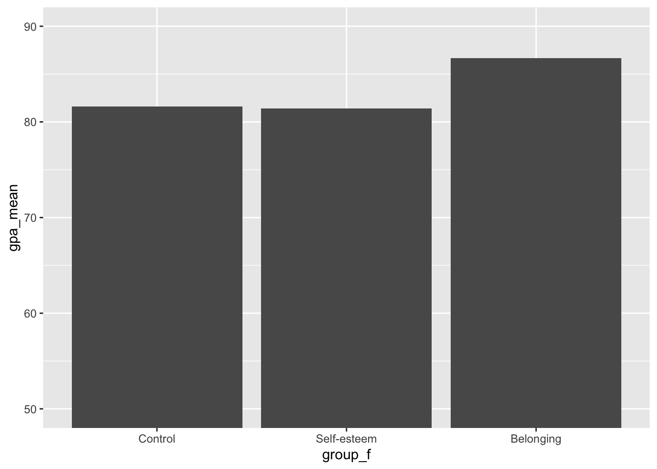

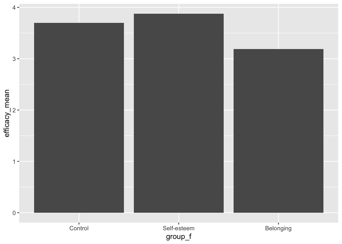
bl_means %>%
  ggplot(aes(x = group_f, y = efficacy_mean)) +
  geom_col()

Our plots might be a bit more informative, though, if we add error bars (in this case, standard deviations). What happens if we add error bars?

bl_means %>%
  ggplot(aes(x = group_f, y = gpa_mean)) +
  geom_col() +
  geom_errorbar(aes(ymin=gpa_mean-gpa_sd, ymax=gpa_mean+gpa_sd), width=.2) +
  coord_cartesian(ylim = c(50, 100))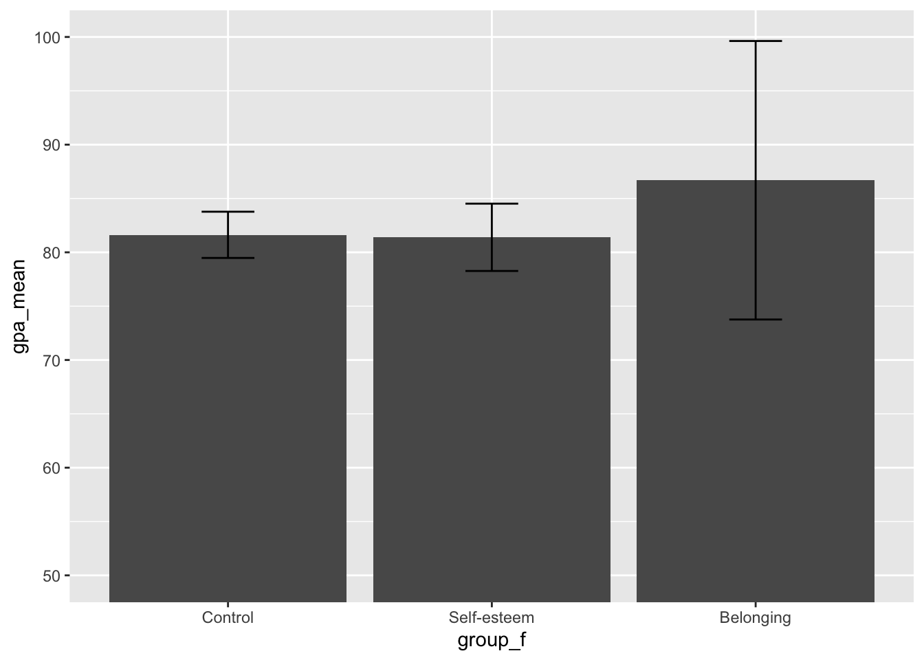

bl_means %>%
  ggplot(aes(x = group_f, y = efficacy_mean)) +
  geom_col() +
  geom_errorbar(aes(ymin=efficacy_mean-efficacy_sd, ymax=efficacy_mean+efficacy_sd), width=.2)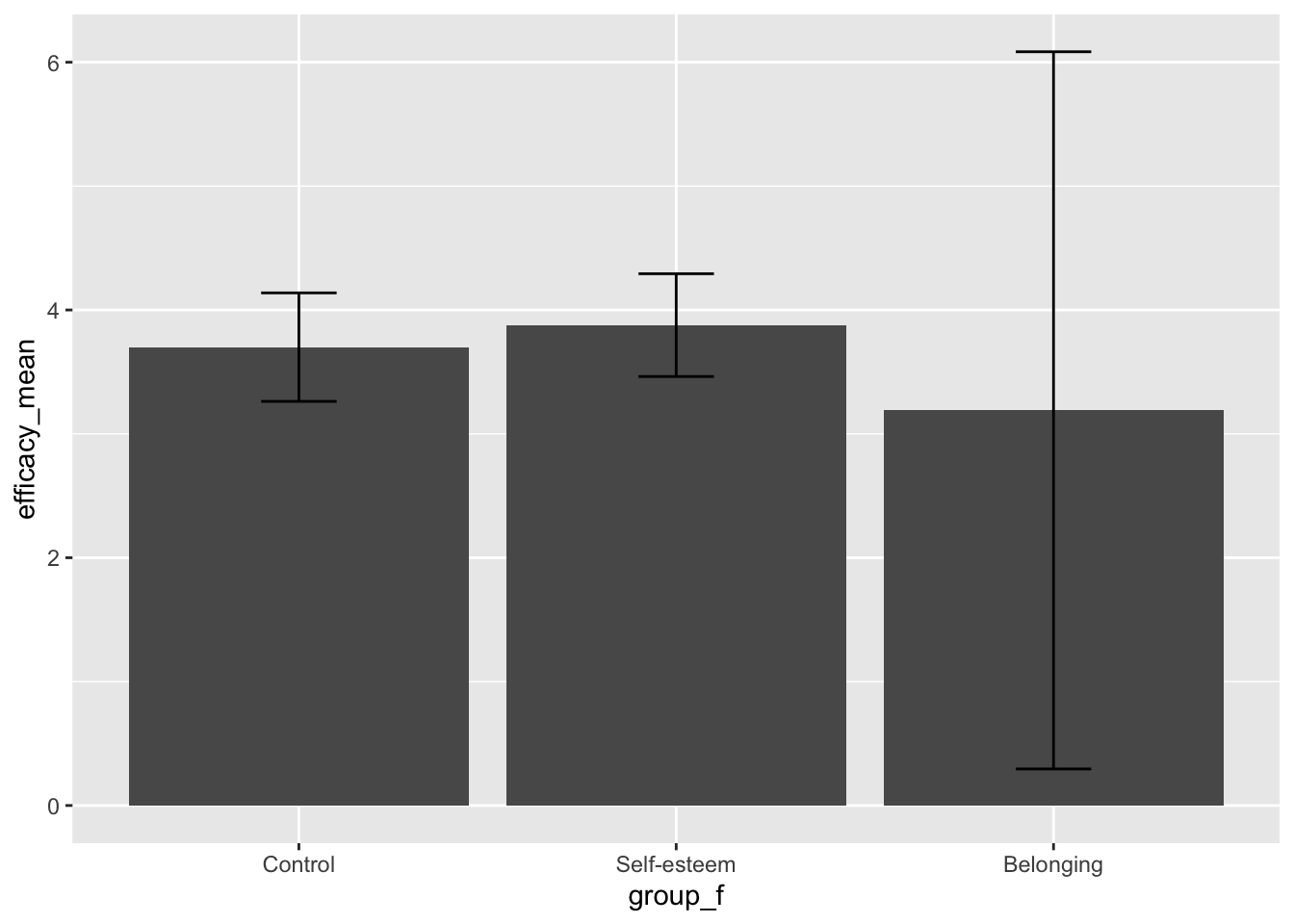

The plot thickens. Adding error bars reveals that there is huge variability in both the GPA and efficacy estimates for the belonging group. What does this mean?

Well, it could mean that there is naturally way more variability in the belonging group across outcomes–rotten luck. That would mean that we failed to randomize the groups properly, and there were baseline differences across groups. When you randomize, you want all groups to be equal across everything–except what you’re manipulating (i.e. the intervention).

It could also mean that the belonging intervention is helpful for some, and hurtful for others, and that there is some moderating factor that determines whether its good or bad. This would also not be ideal–like I said, we don’t want our interventions to ever be hurtful.

But, there’s one other possible explanation: outliers. How could outliers be a problem? and what is an outlier?

5.3 Outliers

5.3.1 What is an outlier?

An outlier is a response (aka data point) that is so far away from the majority of responses for a population or variable that it is considered extreme.

5.3.2 What’s the problem with outliers?

Is that such a bad thing? Why can’t we just leave outliers alone to live their life of solitude on the edges of our data?

Here are 3 problems outliers can create:

They bias or influence estimates of analyses. This can be especially problematic if they substantially influence answers to questions of interest.
They increase error variance and reduce statistical power (aka your likelihood of finding an effect if there is really one there).
They can change the odds of making both type I and type II errors. (See this paper for an example.)

How do they do all of these horrible things?

Let’s look at an example. Run the chunk below and look at the graph. We have 6 data points, with their average represented with the red dot and one standard deviation above and below the mean represented by the red line. Because these data are balanced, the mean represents the typical response of the data, and the standard deviation represents the typical spread perfectly.

dots <- c(5, 6, 5, 6, 5, 6)
num <- c(1, 2, 3, 4, 5, 6)
dotsnum <- cbind.data.frame(dots, num)

dotsnum %>% ggplot(aes(x = num, y = dots)) +
  geom_point() +
  coord_cartesian(ylim = c(1, 10)) +
  xlab("Dot Number") +
  annotate("point", x = mean(num), y = mean(dots), colour = "red", size = 4) +
  annotate("errorbar", x = mean(num), ymin = mean(dots) - sd(dots), ymax = mean(dots) + sd(dots), width = .001, colour = "red")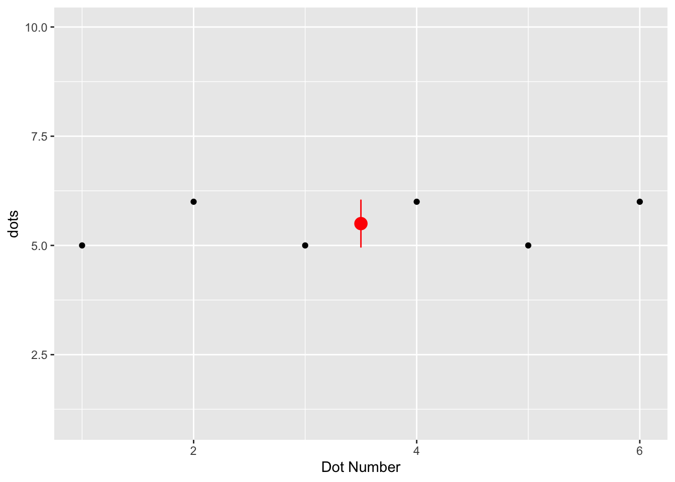

But what happens if one of the responses is far away from the others?

dots <- c(5, 1, 5, 6, 5, 6)
num <- c(1, 2, 3, 4, 5, 6)
dotsnum <- cbind.data.frame(dots, num)

dotsnum %>% ggplot(aes(x = num, y = dots)) +
  geom_point() +
  coord_cartesian(ylim = c(1, 10)) +
  xlab("Dot Number") +
  annotate("point", x = mean(num), y = mean(dots), colour = "red", size = 4) +
  annotate("errorbar", x = mean(num), ymin = mean(dots) - sd(dots), ymax = mean(dots) + sd(dots), width = .001, colour = "red") +
  annotate("point", x = mean(num), y = 5.5, colour = "lightsalmon1", size = 4)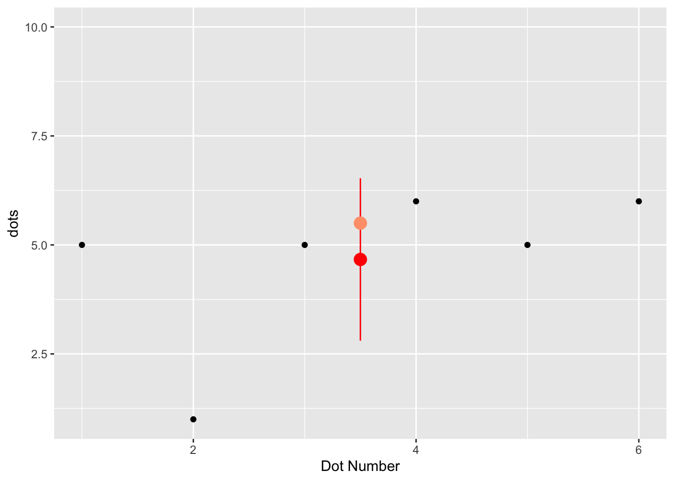

Now, we can see that the new mean has been weighted toward the outlying response, and no longer represents the typical response, indicated by the lighter red (or more specifically “lightsalmon1”) dot that is the mean from the last graph. Even more, the standard deviation is inflated and no longer represents the typical spread of the data, either.

What does this tell us? Outliers disproportionately influence these estimates of central tendency and spread, skewing and inflating them much more than the addition of one “normal” data point would.

Practically speaking, this means that if we have outliers, then:

averages and estimates of relationships (e.g. correlation/regression) will be skewed from the true average or estimate of the underlying population and
measures of variance (including standard deviations and standard errors) will be inflated, making our estimates much less precise, and making it much more difficult to find an effect.

5.3.3 Where do outliers come from?

When we collect data and run analyses, we are sampling (aka taking a few people) from a larger population that we’d like to study. Outliers are problematic in part because they don’t accurately represent the population we would like to study, and therefore make it more difficult to get accurate and precise estimates of what is true for that population, on average.

Here are 3 main types of outliers:

Data errors - Does not represent a true response. Sometimes, we have extreme values from data error. Say, for example, that instead of a 5/5 on the efficacy scale, someone (somehow), scored a 50/5 on the efficacy scale. Data errors like this often create scores outside of the possible range of a variable.
Legitimate data from the wrong population - sampling from people you don’t mean to sample. Sometimes we may unknowingly include someone who is not from the population we wish to study, and they become outliers. For example, say we are interested in how many practice interviews Wharton freshman have done in their first year, but we accidentally include a senior Wharton student in the sample. This student is likely to have much more experience, and probably more extreme responses, compared to our freshman sample. Another example might be accidentally sampling people on an unusual day, such as the day of an important national event. We meant to sample people from normal circumstances, and unusual circumstances may make for unusual responses.
Legitimate data from the right population - extreme responses from people you meant to sample. Sometimes, we get legitimate responses from the right people and they are still extreme responses. Actually, we might expect this! Assuming our data are normally distributed, about 1% of responses are expected to be far away enough from the mean to be outliers. Even though these are legitimate responses and may warrant study in and of themselves, they may still skew estimates for our analyses of the group as a whole, and may need to be addressed.

5.3.4 Univariate outliers

Now that we’ve learned a little bit about outliers and why they may be problematic, how might this apply to our earlier problem with our belonging intervention?

The presence of outliers seems like a reasonable explanation for our problems. If you remember, our data had unexpected means and very inflated standard deviations. If outliers are the culprit, then we might expect that they come from data entry errors; people we didn’t mean to sample; or extreme, but legitimate responses.

Let’s check it out.

At the most basic level, we can check for outliers using boxplots. Because we noticed abnormalities in the outcomes (efficacy and gpa) across intervention groups, let’s plot boxplots for the outcomes across groups.

Boxplots identify outliers with dots beyond the common range of values. Looking at these can show us quickly if there seem to be any extreme scores.

What do you see?

bl %>% ggplot() +
  geom_boxplot(aes(x = group_f, y = efficacy))

bl %>% ggplot() +
  geom_boxplot(aes(x = group_f, y = gpa))

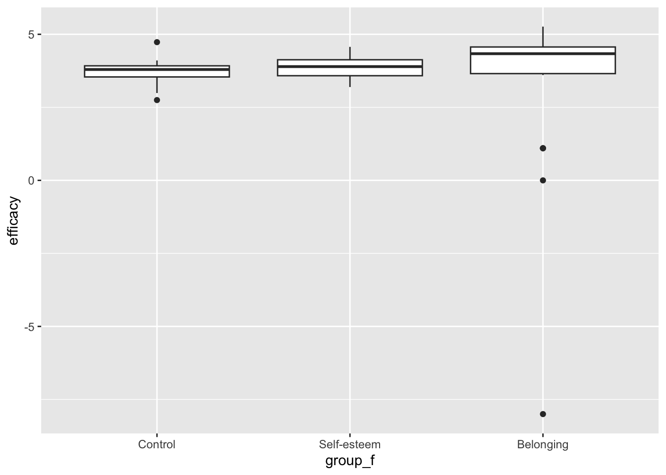
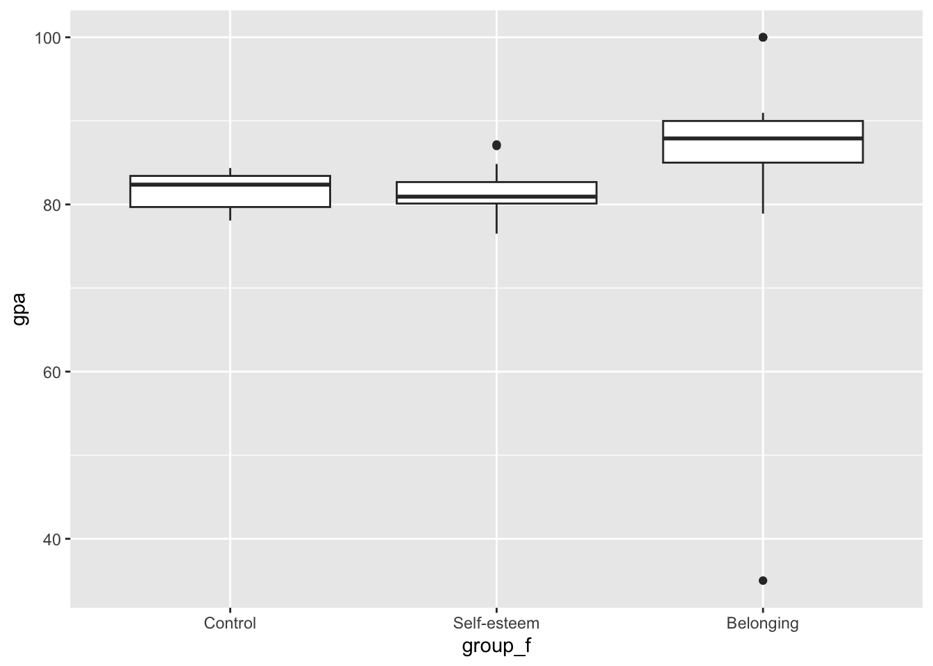
Because we know that the range of possible values for efficacy is 1 - 5, there may be a couple of out-of-bounds responses for efficacy that are causing problems.

Also, because the range for gpa is 50 - 100 (these schools don’t give grades below 50), then it looks like there is an out-of-bounds value for gpa, too. We can quickly see which values might be out-of-bounds using dplyr’s ever-useful filter function:

bl %>% select(id, efficacy) %>% filter(efficacy < 1)

##    id efficacy
## 1 304        0
## 2 305       -8

bl %>% select(id, gpa) %>% filter(gpa < 50)

##    id gpa
## 1 302  35

It looks like our suspicions were correct, and there are two out-of-bounds values for efficacy and one for gpa. Because these are most likely data entry errors and not legitimate responses, we will not consider them in our analyses, and can essentially “delete” them. We will do this by coding them as missing (NA in R means missing). We can do so by recoding our variables to code as missing any values that are out-of-bounds.

#the function ifelse() works like this: ifelse(if_condition, then_do_this, otherwise_do_this). So here, the first one would be read as: "if efficacy is less than one, then code as missing, otherwise code the same as the original efficacy variable".

bl2 <- bl %>% mutate(
  
  efficacy = ifelse(efficacy < 1, NA, efficacy),
  gpa = ifelse(gpa < 50, NA, gpa)
  
)

Now that we have removed the data errors, let’s look at the boxplots again:

bl2 %>% ggplot() +
  geom_boxplot(aes(x = group_f, y = efficacy))

## Warning: Removed 2 rows containing non-finite outside the scale range
## (`stat_boxplot()`).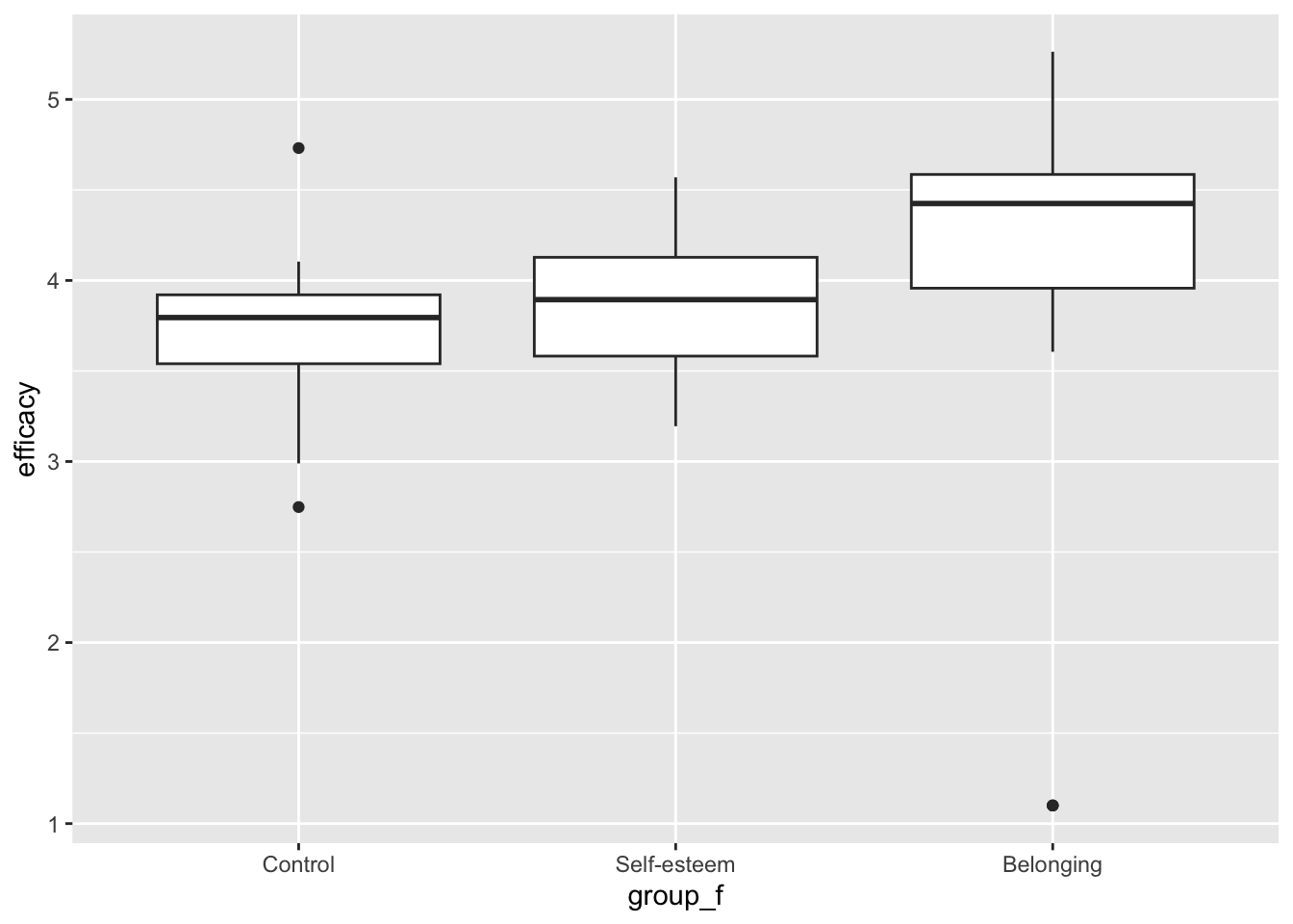

bl2 %>% ggplot() +
  geom_boxplot(aes(x = group_f, y = gpa))

## Warning: Removed 1 row containing non-finite outside the scale range
## (`stat_boxplot()`).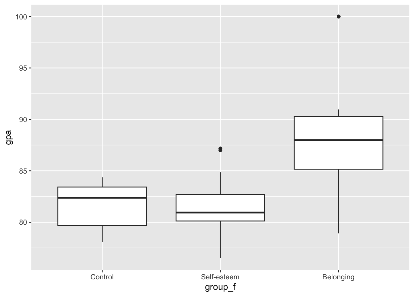

It looks like there still might be a few outliers. Because we have already dealt with suspected data entry errors, we will assume that the remaining outliers are legitimate, but extreme responses. At this point, unfortunately, it’s difficult to tell what causes these outliers, so we will treat them all the same.

To deal with these outliers, we’ll use one of the most basic (and conservative) methods for dealing with outliers: the z-score method.

The z-score method excludes any values above or below 3 standard deviations from the mean. To do this, the first step is to identify if there are any values beyond this threshold. filter, again, is a great way to do this:

bl2 %>% 
  select(id, gpa) %>% 
  mutate(z_gpa = as.numeric(scale(gpa))) %>% 
  filter(z_gpa>=3| z_gpa<=-3)

## [1] id    gpa   z_gpa
## <0 rows> (or 0-length row.names)

bl2 %>% 
  select(efficacy) %>% 
  mutate(z_efficacy = as.numeric(scale(efficacy))) %>% 
  filter(z_efficacy>=3 | z_efficacy<=-3)

##   efficacy z_efficacy
## 1      1.1  -3.292483
## 2      1.1  -3.292483
## 3      1.1  -3.292483

It looks like there are 3 values of efficacy that are more than 3 standard deviations below the mean (scale(efficacy) < -3). Using the code below, let’s recode those values to be missing.

bl2.no.out <- bl2 %>% mutate(
  
  efficacy = ifelse(scale(efficacy) < -3, 
                NA,
                efficacy)
  
)

Now that we’ve taken care of outliers, let’s look at the effect of the intervention on efficacy and gpa again.

bl_means <- bl2.no.out %>% 
              group_by(group_f) %>% 
                summarise(gpa_mean = mean(gpa, na.rm = TRUE), 
                          gpa_sd = sd(gpa, na.rm = TRUE), 
                          efficacy_mean = mean(efficacy, na.rm = TRUE), 
                          efficacy_sd = sd(efficacy, na.rm = TRUE))

bl_means %>%
  ggplot(aes(x = group_f, y = gpa_mean)) +
  geom_col() +
  geom_errorbar(aes(ymin=gpa_mean-gpa_sd, ymax=gpa_mean+gpa_sd), width=.2) +
  coord_cartesian(ylim = c(50, 100))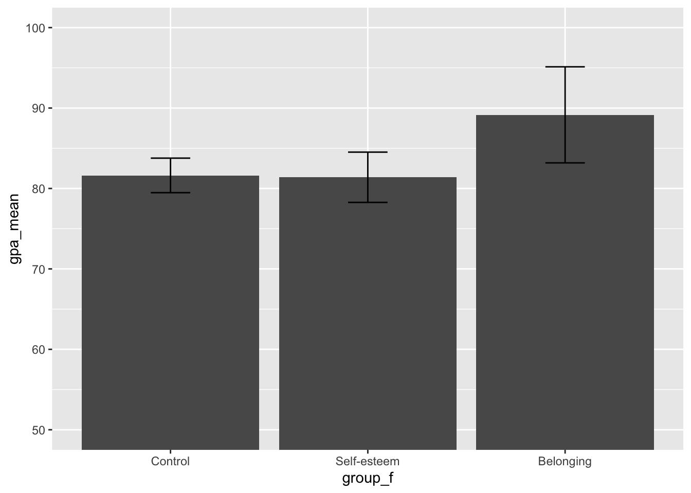

bl_means %>%
  ggplot(aes(x = group_f, y = efficacy_mean)) +
  geom_col() +
  geom_errorbar(aes(ymin=efficacy_mean-efficacy_sd, ymax=efficacy_mean+efficacy_sd), width=.2)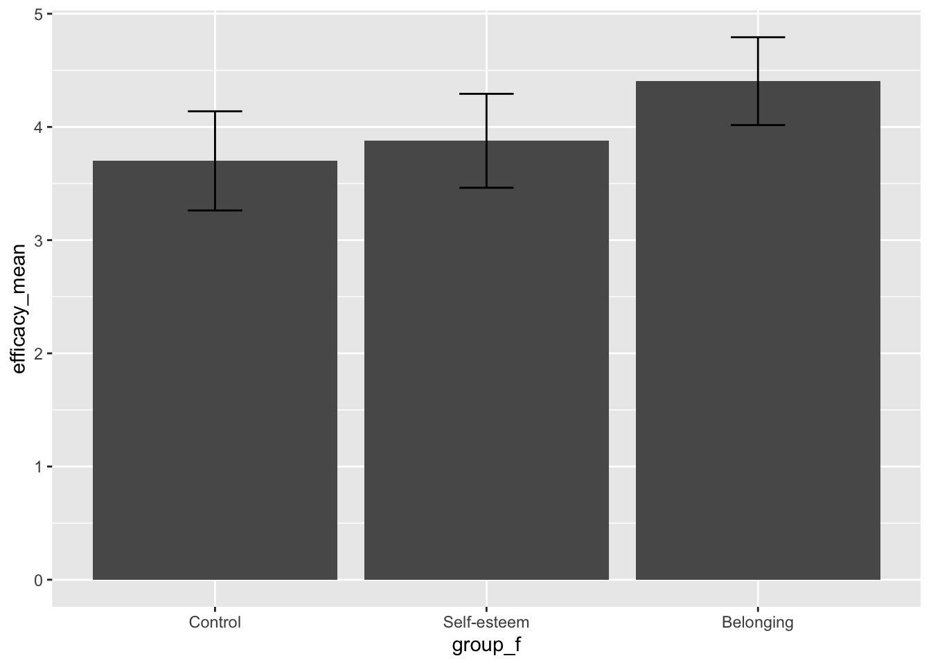

We can see that removing outliers significantly increased the average score of efficacy in the belonging condition; Also, the variability in both gpa and efficacy is much lower. Removing outliers helped correct skewed means and make estimates of variability more precise.

5.3.5 Multivariate outliers

When you have a larger dataset, using univariate outliers can get annoying quickly:

Scanning each variable takes a lot of time
Even if you wrote code to do it faster, you might end up eliminating too much data

What happens if we want to see if there are outliers on more than two dimensions or variables? Well, we wouldn’t be able to visualize it well, because there isn’t a good way to graph anything larger than 3 dimensions. We definitely can’t just take the z-score, because we don’t have a z-score that takes into account more than one dimension… If we could only compute some sort of measurement that tells us how different a person’s overall response is compared to everyone else… Wait! We do have something like a z-score that works for many dimensions: Mahalanobis distance.

Disregarding how hard that is to say, Mahalanobis distance is doing essentially the same thing as a z-score: taking an average and computing how far away something is from that average. Like a z-score, things that are very far away would be considered outliers. However, instead of looking at the average of a single variable, like a z-score, Mahalanobis distance assesses the average pattern of responses across many variables, and subsequently computes the distance of each individual’s pattern of response from the average pattern.

Mahalanobis distances also solve one issue of working with multiple variables: The correlation problem. Why would correlation be a problem in outlier detection? See the following plot:

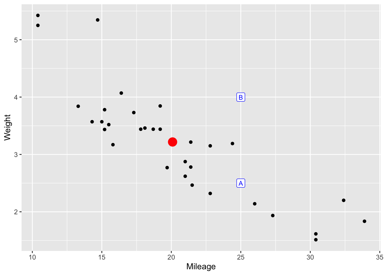
Check out Points A and B. They are the same distance from the mean of weight and mileage (About an inch, using my ruler), yet, point B is much more likely an outlier than point A. That’s because, in order to accurately calculate multivariate outliers, we need to take into account the correlation between weight and mileage.

This is essentially what Mahalanobis Distances are doing with as many variables as you would like to include. They are comparing each of the rows in your data set (each survey response, for example), with everybody else’s responses. Taking correlation into account, it generates one number that represents how far away that response is from all others.

PS: If you thought this was incredibly interesting, here is a youtube video going into more detail.

5.3.5.1 How do we compute multivariate outliers?

We can then test these distances for statistical significance; in line with a common standard of Mahalanobis distances, we’ll say anyone whose distance is a .001 probability of occurring an outlier.

This is exactly what this custom function (MO_Detection) is doing:

Generates a mean vector and a covariance matrix (think correlation matrix) from the data
Inputs those to generate a vector of Mahalanobis distances
Calculates what the cutoff would be to exclude cases where the distance is p < .001, using the chi-squared distribution and the number of variables
Returns a plot and a data frame without the outliers.

This whole procedure and function was inspired and adapted from this video. (Thanks Dr. Buchanan!)

MO_Detection = function (CompleteDataset, AnalyzedDataset, alpha = 0.001) {
  Means = colMeans(AnalyzedDataset, na.rm = T)
  Covariance = cov(AnalyzedDataset, use = "pairwise.complete.obs")
  Distances = mahalanobis(AnalyzedDataset, Means, Covariance)
  cutoff = qchisq(1-alpha, ncol(AnalyzedDataset))
  remain = Distances < cutoff
  PlotData = AnalyzedDataset %>% 
    mutate(ID = 1:nrow(AnalyzedDataset), 
           Distance = Distances, 
           # state both levels explicitly, so this still works when every case
           # falls on the same side of the cutoff
           Outlier = factor(remain, levels = c(FALSE, TRUE), labels = c("Yes","No")))
  n = nrow(AnalyzedDataset) - sum(remain)
  report = paste(n, "cases were multivariate outliers")
  print(report)
  p = ggplot(PlotData, aes(ID, Distance, color = Outlier)) + 
    geom_point() + 
    labs(title = "Multivariate Outliers",
         subtitle = report) +
    theme(legend.position = "bottom")
  print(p)

  return(CompleteDataset %>% filter(remain))
}

Let’s try removing multivariate outliers from our Belonging Intervention Study. The MO_Detection function takes as input the complete dataset, the dataset with the variables we’ll use (only numeric variables), and the alpha level (set as default at the .001 level).

bl_noout = MO_Detection(bl, bl[7:9])

## [1] "2 cases were multivariate outliers"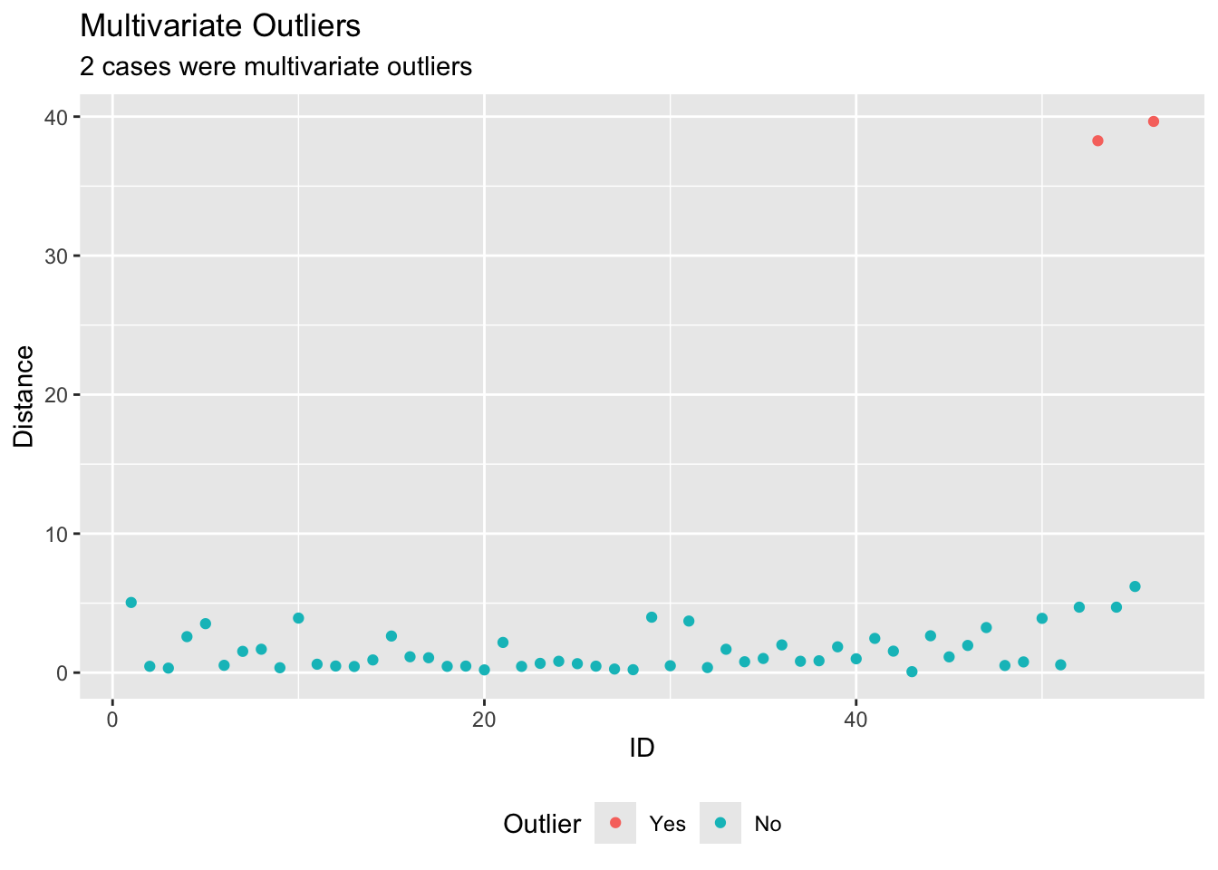

Practice

Try changing the alpha value to something even more improbable (say .00000000001), or more probable (say .30), and see how that changes how many cases are flagged as outliers. (Note that .001 is customary.)

Answer

MO_Detection(bl, bl[7:9], alpha = .00000000001)  # far stricter

## [1] "0 cases were multivariate outliers"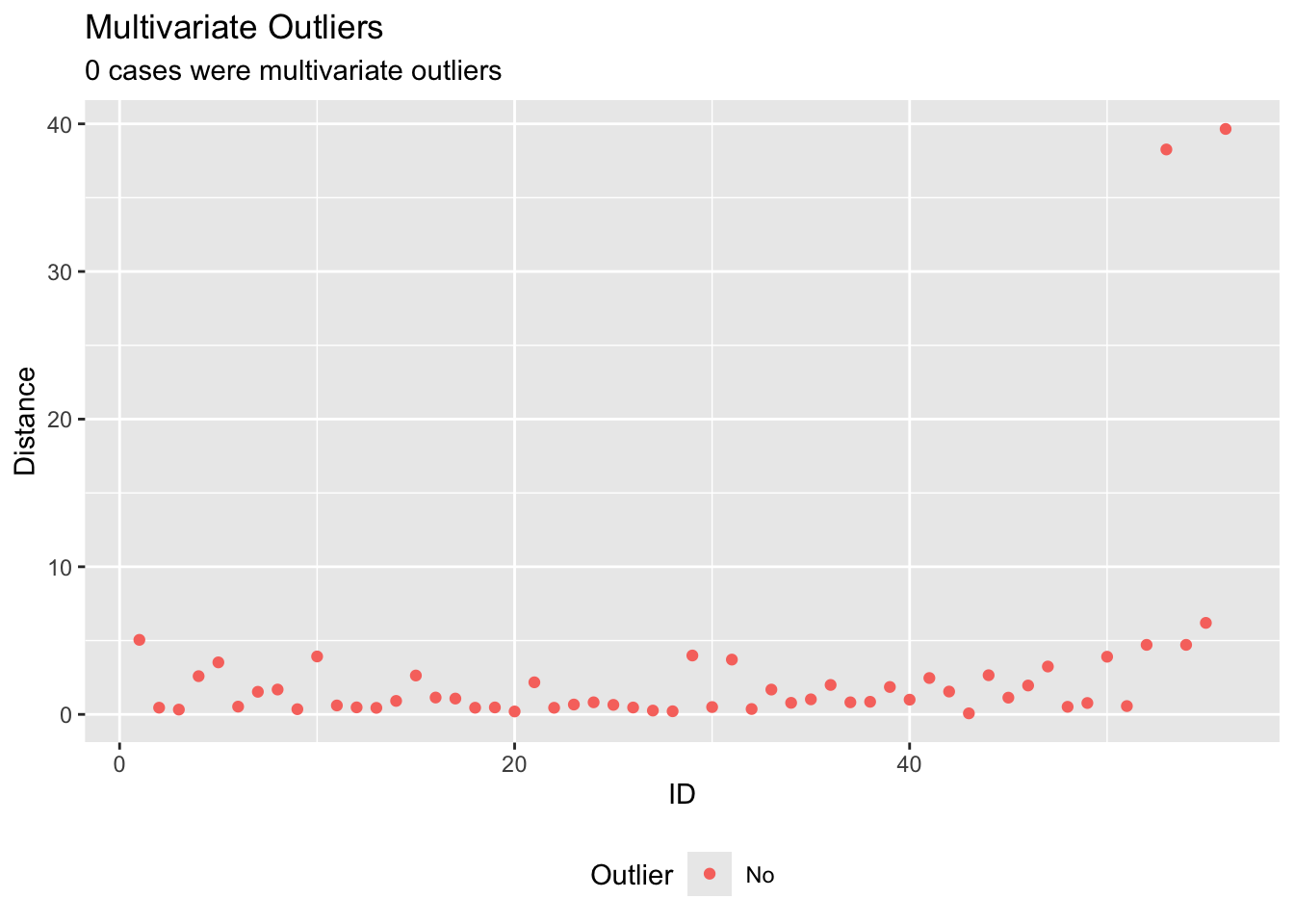

##      X  id                school_f      age gender_f     group_f       gpa
## 1  250 250   Jefferson High School 17.39187   Female     Control  83.41747
## 2  251 251   Jefferson High School 14.18992     Male Self-esteem  78.83002
## 3  252 252 Summerfield High School 15.18526     Male   Belonging  84.11097
## 4  253 253   Jefferson High School 14.79946     Male     Control  78.07654
## 5  254 254   Jefferson High School 11.36432     Male Self-esteem  80.93399
## 6  255 255   Jefferson High School 16.66312     Male   Belonging  88.01059
## 7  256 256 Summerfield High School 15.75501     Male     Control  83.28345
## 8  257 257   Jefferson High School 14.75643     Male Self-esteem  80.55490
## 9  258 258 Summerfield High School 13.01375   Female   Belonging  78.90696
## 10 259 259        Alta High School 17.93749     Male     Control  84.36147
## 11 260 260 Summerfield High School 14.99032   Female Self-esteem  84.84585
## 12 261 261 Summerfield High School 16.24484     Male   Belonging  85.39739
## 13 262 262 Summerfield High School 19.13195   Female     Control  78.27902
## 14 263 263 Summerfield High School 14.32676     Male Self-esteem  82.10003
## 15 264 264   Jefferson High School 15.00327   Female   Belonging  87.82432
## 16 265 265   Jefferson High School 16.03146     Male     Control  83.66960
## 17 266 266 Summerfield High School 15.66807   Female Self-esteem  87.17029
## 18 267 267   Jefferson High School 14.93634     Male   Belonging  84.95335
## 19 268 268 Summerfield High School 16.35058   Female     Control  82.37217
## 20 269 269        Alta High School 16.66361   Female Self-esteem  87.00253
## 21 270 270        Alta High School 13.76062     Male   Belonging  84.79597
## 22 271 271   Jefferson High School 12.58009     Male     Control  80.83171
## 23 272 272 Summerfield High School 16.04535     Male Self-esteem  77.68560
## 24 273 273        Alta High School 14.74291   Female   Belonging  88.36227
## 25 274 274 Summerfield High School 13.24099   Female     Control  79.57642
## 26 275 275        Alta High School 17.67707     Male Self-esteem  80.22519
## 27 276 276   Jefferson High School 16.09295     Male   Belonging  85.16007
## 28 277 277        Alta High School 14.53651   Female     Control  82.83351
## 29 278 278   Jefferson High School 16.22282   Female Self-esteem  76.51259
## 30 279 279        Alta High School 18.68051   Female   Belonging  86.22347
## 31 280 280   Jefferson High School 16.92381   Female     Control  78.45885
## 32 281 281        Alta High School 13.20724     Male Self-esteem  80.11364
## 33 282 282        Alta High School 15.28673   Female   Belonging  88.92390
## 34 283 283        Alta High School 16.19274     Male     Control  82.55526
## 35 284 284 Summerfield High School 12.87938     Male Self-esteem  82.67894
## 36 285 285        Alta High School 15.75797   Female   Belonging  89.11255
## 37 286 286        Alta High School 15.12257   Female     Control  79.69369
## 38 287 287        Alta High School 14.62111     Male Self-esteem  76.93011
## 39 288 288   Jefferson High School 17.22538     Male   Belonging  90.96326
## 40 289 289        Alta High School 15.67515     Male     Control  80.80792
## 41 290 290        Alta High School 17.23564     Male Self-esteem  81.90473
## 42 291 291   Jefferson High School 16.24451   Female   Belonging  87.97255
## 43 292 292 Summerfield High School 14.10102   Female     Control  83.79780
## 44 293 293 Summerfield High School 15.57494   Female Self-esteem  84.27826
## 45 294 294 Summerfield High School 16.26866   Female   Belonging  90.28180
## 46 295 295        Alta High School 15.51091     Male     Control  81.63840
## 47 296 296 Summerfield High School 18.34475   Female Self-esteem  81.48714
## 48 297 297   Jefferson High School 17.27340   Female   Belonging  86.59865
## 49 298 298        Alta High School 19.31548     Male     Control  83.96875
## 50 299 299 Summerfield High School 17.46790   Female Self-esteem  80.45219
## 51 300 300 Summerfield High School 19.42146     Male   Belonging  84.63917
## 52 301 301 Summerfield High School 19.42146   Female   Belonging 100.00000
## 53 302 302        Alta High School 19.42146     Male   Belonging  35.00000
## 54 303 303   Jefferson High School 19.42146   Female   Belonging 100.00000
## 55 304 304 Summerfield High School 19.42146     Male   Belonging 100.00000
## 56 305 305 Summerfield High School 19.42146     Male   Belonging 100.00000
##     efficacy      swb
## 1   3.921683 4.169868
## 2   3.875573 6.050384
## 3   4.514029 5.843839
## 4   3.920615 4.720602
## 5   3.763534 7.088708
## 6   3.799149 5.439898
## 7   3.380281 4.905622
## 8   4.425272 6.587388
## 9   4.168337 5.678804
## 10  3.855377 4.361223
## 11  3.910569 6.276172
## 12  4.605736 5.860298
## 13  3.540068 5.623322
## 14  3.980757 6.414969
## 15  3.605931 4.670073
## 16  3.807990 5.012063
## 17  3.774733 6.415198
## 18  4.523294 5.513297
## 19  2.989357 5.387003
## 20  3.582126 5.648929
## 21  4.657245 6.667443
## 22  3.453221 5.372424
## 23  4.270552 6.028213
## 24  4.579443 5.597670
## 25  3.831375 5.304716
## 26  4.569605 5.952221
## 27  4.281616 5.627244
## 28  4.104148 5.506344
## 29  4.127815 7.059081
## 30  4.512180 5.880012
## 31  3.655640 4.477502
## 32  3.250539 6.061472
## 33  5.263224 5.451290
## 34  3.541798 5.153664
## 35  4.111012 6.439699
## 36  4.118973 6.576066
## 37  3.936328 5.214086
## 38  3.410356 5.469156
## 39  4.603518 6.238228
## 40  2.748390 5.246290
## 41  3.893987 6.867788
## 42  4.783218 5.143209
## 43  3.795007 5.605537
## 44  3.194834 6.936671
## 45  4.459572 5.530439
## 46  4.731285 4.850798
## 47  4.392256 6.981173
## 48  4.009894 5.374307
## 49  3.689712 5.148220
## 50  3.388009 7.164033
## 51  4.390583 6.134025
## 52  1.100000 6.134025
## 53  1.100000 6.134025
## 54  1.100000 6.134025
## 55  0.000000 6.134025
## 56 -8.000000 6.134025

MO_Detection(bl, bl[7:9], alpha = .30)           # far looser

## [1] "10 cases were multivariate outliers"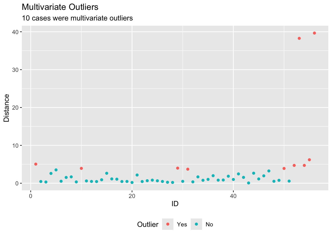

##      X  id                school_f      age gender_f     group_f      gpa
## 1  251 251   Jefferson High School 14.18992     Male Self-esteem 78.83002
## 2  252 252 Summerfield High School 15.18526     Male   Belonging 84.11097
## 3  253 253   Jefferson High School 14.79946     Male     Control 78.07654
## 4  254 254   Jefferson High School 11.36432     Male Self-esteem 80.93399
## 5  255 255   Jefferson High School 16.66312     Male   Belonging 88.01059
## 6  256 256 Summerfield High School 15.75501     Male     Control 83.28345
## 7  257 257   Jefferson High School 14.75643     Male Self-esteem 80.55490
## 8  258 258 Summerfield High School 13.01375   Female   Belonging 78.90696
## 9  260 260 Summerfield High School 14.99032   Female Self-esteem 84.84585
## 10 261 261 Summerfield High School 16.24484     Male   Belonging 85.39739
## 11 262 262 Summerfield High School 19.13195   Female     Control 78.27902
## 12 263 263 Summerfield High School 14.32676     Male Self-esteem 82.10003
## 13 264 264   Jefferson High School 15.00327   Female   Belonging 87.82432
## 14 265 265   Jefferson High School 16.03146     Male     Control 83.66960
## 15 266 266 Summerfield High School 15.66807   Female Self-esteem 87.17029
## 16 267 267   Jefferson High School 14.93634     Male   Belonging 84.95335
## 17 268 268 Summerfield High School 16.35058   Female     Control 82.37217
## 18 269 269        Alta High School 16.66361   Female Self-esteem 87.00253
## 19 270 270        Alta High School 13.76062     Male   Belonging 84.79597
## 20 271 271   Jefferson High School 12.58009     Male     Control 80.83171
## 21 272 272 Summerfield High School 16.04535     Male Self-esteem 77.68560
## 22 273 273        Alta High School 14.74291   Female   Belonging 88.36227
## 23 274 274 Summerfield High School 13.24099   Female     Control 79.57642
## 24 275 275        Alta High School 17.67707     Male Self-esteem 80.22519
## 25 276 276   Jefferson High School 16.09295     Male   Belonging 85.16007
## 26 277 277        Alta High School 14.53651   Female     Control 82.83351
## 27 279 279        Alta High School 18.68051   Female   Belonging 86.22347
## 28 281 281        Alta High School 13.20724     Male Self-esteem 80.11364
## 29 282 282        Alta High School 15.28673   Female   Belonging 88.92390
## 30 283 283        Alta High School 16.19274     Male     Control 82.55526
## 31 284 284 Summerfield High School 12.87938     Male Self-esteem 82.67894
## 32 285 285        Alta High School 15.75797   Female   Belonging 89.11255
## 33 286 286        Alta High School 15.12257   Female     Control 79.69369
## 34 287 287        Alta High School 14.62111     Male Self-esteem 76.93011
## 35 288 288   Jefferson High School 17.22538     Male   Belonging 90.96326
## 36 289 289        Alta High School 15.67515     Male     Control 80.80792
## 37 290 290        Alta High School 17.23564     Male Self-esteem 81.90473
## 38 291 291   Jefferson High School 16.24451   Female   Belonging 87.97255
## 39 292 292 Summerfield High School 14.10102   Female     Control 83.79780
## 40 293 293 Summerfield High School 15.57494   Female Self-esteem 84.27826
## 41 294 294 Summerfield High School 16.26866   Female   Belonging 90.28180
## 42 295 295        Alta High School 15.51091     Male     Control 81.63840
## 43 296 296 Summerfield High School 18.34475   Female Self-esteem 81.48714
## 44 297 297   Jefferson High School 17.27340   Female   Belonging 86.59865
## 45 298 298        Alta High School 19.31548     Male     Control 83.96875
## 46 300 300 Summerfield High School 19.42146     Male   Belonging 84.63917
##    efficacy      swb
## 1  3.875573 6.050384
## 2  4.514029 5.843839
## 3  3.920615 4.720602
## 4  3.763534 7.088708
## 5  3.799149 5.439898
## 6  3.380281 4.905622
## 7  4.425272 6.587388
## 8  4.168337 5.678804
## 9  3.910569 6.276172
## 10 4.605736 5.860298
## 11 3.540068 5.623322
## 12 3.980757 6.414969
## 13 3.605931 4.670073
## 14 3.807990 5.012063
## 15 3.774733 6.415198
## 16 4.523294 5.513297
## 17 2.989357 5.387003
## 18 3.582126 5.648929
## 19 4.657245 6.667443
## 20 3.453221 5.372424
## 21 4.270552 6.028213
## 22 4.579443 5.597670
## 23 3.831375 5.304716
## 24 4.569605 5.952221
## 25 4.281616 5.627244
## 26 4.104148 5.506344
## 27 4.512180 5.880012
## 28 3.250539 6.061472
## 29 5.263224 5.451290
## 30 3.541798 5.153664
## 31 4.111012 6.439699
## 32 4.118973 6.576066
## 33 3.936328 5.214086
## 34 3.410356 5.469156
## 35 4.603518 6.238228
## 36 2.748390 5.246290
## 37 3.893987 6.867788
## 38 4.783218 5.143209
## 39 3.795007 5.605537
## 40 3.194834 6.936671
## 41 4.459572 5.530439
## 42 4.731285 4.850798
## 43 4.392256 6.981173
## 44 4.009894 5.374307
## 45 3.689712 5.148220
## 46 4.390583 6.134025

At the customary .001 we flag 2 cases. Make alpha far stricter and we flag none at all; loosen it to .30 and we flag 10. A stricter alpha means a case has to be more extreme before we are willing to call it an outlier–which is why the conventional cutoff matters, and why you should not go fishing for the alpha that gives you the answer you want.

5.4 Reliability

After we take care of outliers, another very important issue is measurement, what we call psychometrics. One of the most important psychometric properties of our data is reliability.

For reliability discussion today, let’s talk (and learn how to compute) Cronbach’s Alpha.

In psychology, we often use self-report scales with multiple items; create composites of those scales; and measure “reliability” of those scales using Cronbach’s Alpha. However, most people have a hard time articulating what Cronbach’s Alpha actually means. What is Cronbach’s Alpha actually measuring? What does it mean to be “reliable”? How do you compute Cronbach’s alpha in R? And how do you interpret it?

Let’s dive in.

First, what is Cronbach’s Alpha actually measuring?

Let’s look at an example that might help.

First, load in the data. Also, if you haven’t already, load in the package psych.

bl.full <- read.csv("belonging study.csv")

For simplicity, let’s only keep the variables that we will be using for our alpha calculation: efficacy items. One slick way to do this is to use select from dplyr in conjunction with the helper function starts_with:

bl.full %<>% select(starts_with("efficacy"))

Computing Cronbach’s alpha in R is simple. Just use the function alpha from the psych package, and insert your data you want analyzed as the argument. Here, let’s save the output as an object called efficacy.a, then take a look.

efficacy.a <- alpha(bl.full)

## Number of categories should be increased  in order to count frequencies.

efficacy.a

## 
## Reliability analysis   
## Call: alpha(x = bl.full)
## 
##   raw_alpha std.alpha G6(smc) average_r S/N    ase mean   sd median_r
##        0.9       0.9    0.88       0.7 9.3 0.0091  3.9 0.62      0.7
## 
##     95% confidence boundaries 
##          lower alpha upper
## Feldt     0.88   0.9  0.92
## Duhachek  0.89   0.9  0.92
## 
##  Reliability if an item is dropped:
##           raw_alpha std.alpha G6(smc) average_r S/N alpha se   var.r med.r
## efficacy1      0.87      0.87    0.81      0.69 6.6    0.013 1.3e-04  0.68
## efficacy2      0.88      0.88    0.83      0.71 7.2    0.012 9.7e-04  0.70
## efficacy3      0.88      0.88    0.83      0.71 7.2    0.012 1.0e-03  0.70
## efficacy4      0.87      0.87    0.82      0.70 7.0    0.013 2.0e-06  0.70
## 
##  Item statistics 
##             n raw.r std.r r.cor r.drop mean   sd
## efficacy1 300  0.89  0.89  0.84   0.80  3.9 0.73
## efficacy2 300  0.87  0.87  0.81   0.77  3.9 0.68
## efficacy3 300  0.87  0.87  0.81   0.77  3.9 0.69
## efficacy4 300  0.88  0.88  0.83   0.78  3.9 0.72

Yikes–that’s a lot to look at, and we don’t even know what 95% of it means! In a few minutes I’ll show you a custom function that is much more user friendly, but for now, here’s the alpha:

efficacy.a$total$raw_alpha

## [1] 0.9030008

5.4.1 What is alpha actually measuring? How do you compute alpha?

It’s actually pretty simple. Here’s the formula for Cronbach’s alpha:

$\frac{k\bar{r}}{1+(k - 1)\bar{r}}$

where:

k = the number of items
$\bar{r}$ = the average inter-item correlation

That’s not so hard–it really only needs two numbers to work. But what exactly is the “average inter-item correlation”?

Here’s an explanation: Take the first item of our scale, “efficacy1”, correlate it with each other item–“efficacy2”, “efficacy3”, and “efficacy4”–and average those correlations, and we have the average inter-item correlation for “efficacy1”. If we then take the average inter-item correlation for each item and average those together, we get the average inter-item correlation for the scale, what we are calling here $\bar{r}$.

To put it into words, computing Cronbach’s alpha is multiplying the number of items by the average inter-item correlation, then dividing that by the same average correlation scaled up by the number of items–which is what the $1+(k - 1)\bar{r}$ in the denominator is doing. The effect is that alpha rises both when items correlate more strongly and when you add more items.

So, we could say Cronbach’s alpha is the proportion of the total variance of the items that is explained across items, or varies together across items.

Let’s try it ourselves and see if we get the same value as the alpha function.

First: we can let alpha do some of the work for us–from the output we can extract the average inter-item correlations.

rbar <- efficacy.a$total$average_r

Second: We have 4 items, so we’ll set k = 4

k <- 4

Third: plug those values into the formula

alpha.by.hand <- (k*rbar)/(1+(k - 1)*rbar)

alpha.by.hand

## [1] 0.903152

Great, we were able to get the result: a = .90! This means that among the total variation in the scores, 90% of the variance is explained by the items in the scale varying together.

And what exactly does it mean to vary together? Really it just means to correlate: when one goes up, the other goes up; when one goes down, the other goes down.

5.4.2 What is a “good” alpha?

The standards for the field (though somewhat arbitrary) are clear: a = .70 is acceptable, a = .80 is good, and a = .90 is great. Anything under a = .65 will generally require a strong rationale for why that level of inconsistency is acceptable.

5.4.3 In sum, what is alpha?

So, Cronbach’s alpha is a measure of consistency of responses in the data among the items of a scale.

The smaller the shared variance is, the higher the error variance, or unexplained variance is. This means that unaccounted variation is playing a bigger part in the measure (if the items are combined), introducing more random noise and inconsistency. Herein, as error variance increases, the composite will be a less consistent measure.

5.4.4 In sum what is alpha not?

Alpha is:

NOT a measure of reliability of the scale. This is a little nitpicky, but alpha is not a measure of reliability of the scale, it is a measure of the reliability (consistency) of responses in your data. Why does that matter? That matters because it means that Cronbach’s alpha is expected to vary across data sets–it shouldn’t (necessarily) be perfectly consistent across data sets because correlations between items will vary. Rather, it is a measure of the consistency of your responses and should be computed for each data set.
NOT a measure of unidimensionality. High alpha does not imply unidimensionality. Actually, multidimensional data can still have an adequate alpha, but on the flip side, Cronbach’s alpha does assume unidimensionality, and thus should not be performed on multidimensional data.
NOT an indication that your items are highly correlated. Importantly, alpha is heavily influenced by number of items as well as correlation strength. For example, 60 items correlated at an average of r = .07 will have an alpha of .82. Another example: we might consider an alpha of .73 acceptable, but for a scale of 5 items, this would mean an average inter-item correlation of only r = .35. Acceptable alpha does not imply high inter-item correlation.
NOT justification for combining scale items into a composite. Factor analysis is better suited for this as it determines underlying factors in the data and gives estimates of the amount of information retained in a composite score from the constituent items.

5.4.5 A function for formatted alpha output

The raw alpha() output we saw above tells us everything, but it takes a lot of squinting. Everything worth reading is in there–we just need to pull out the useful pieces and lay them out. Let’s write a small function that does that.

Don’t worry about understanding every line; the point is that once you know where alpha() keeps its results, you can reshape them however you like.

alpha_table <- function(data, digits = 3) {
  
  a <- psych::alpha(data)   # everything we need is already in here
  
  data.frame(
    Item = rownames(a$item.stats),
    obs  = a$item.stats$n,
    sign = ifelse(a$item.stats$raw.r >= 0, "+", "-"),
    
    # how each item relates to the scale
    `item-test correlation` = round(a$item.stats$r.cor,  digits),
    `item-rest correlation` = round(a$item.stats$r.drop, digits),
    
    # what happens to the scale if we drop that item
    `avg inter-item correlation` = round(a$alpha.drop$average_r,  digits),
    `alpha if dropped`           = round(a$alpha.drop$raw_alpha, digits),
    
    check.names = FALSE, row.names = NULL
  )
}

Now the same analysis reads much more easily:

bl.full %>% alpha_table() %>% knitr::kable()

Item	obs	sign	item-test correlation	item-rest correlation	avg inter-item correlation	alpha if dropped
efficacy1	300	+	0.845	0.802	0.687	0.868
efficacy2	300	+	0.812	0.772	0.707	0.879
efficacy3	300	+	0.813	0.773	0.706	0.878
efficacy4	300	+	0.827	0.785	0.699	0.874

The three middle columns represent the different types of correlations computed, which can be informative, but are not always necessary. Most informative is “alpha if dropped”–this tells you what Cronbach’s alpha would be if you dropped that item from the scale. Here, dropping any single efficacy item would lower alpha, which is a good sign: every item is pulling its weight.

Practice

The swb items in bl.full measure subjective well-being. Compute Cronbach’s alpha for those four items, the same way we just did for efficacy. Is the scale reliable?

Answer

# note: we trimmed bl.full down to the efficacy items earlier, so read the file again
swb_items <- read.csv("belonging study.csv") %>% select(starts_with("swb"))

alpha(swb_items)$total$raw_alpha

## Number of categories should be increased  in order to count frequencies.

## [1] 0.9295663

An alpha of about .93 is well past the .90 “great” threshold–these four items hang together very consistently. Remember that this does not mean the scale is unidimensional; that is what factor analysis is for.

5.5 Factor analysis

So far, we’ve been happily creating composites from items, without putting too much thought into important questions:

Are all these questions related enough to justify adding them together?

Should we add all the items together into a single composite or should we create more composites?

Are all items working properly, or are there some that are not working well?

If we are summarizing ten columns (for ten items), into one (for the composite), how much information are we losing?

Factor analysis, and related techniques, help us answer all of these questions.

Let’s start by loading our data.

sps <- read.csv("Confidence in Science.csv")
# View(sps)

The data (this time it’s real), asks participants for their perception of efficacy of scientific (e.g. medicine) and pseudoscientific practices (e.g. Tarot).

Say we want to work with a smaller number of variables (rather than the full 13), and we think these items represent one or two underlying constructs. Factor analysis will help us make those decisions and justify how we make our composites.

Most likely the items will form a single factor. A continuum starting in complete belief in science and disregard for pseudoscience, and ending in the opposite, people who distrust the scientific establishment in favor of more ‘alternative methods’

Fig 1. A single factor

Here are the steps

5.5.1 Are the items correlated enough to warrant a composite

The first condition is that the items need to be correlated enough to justify adding some of them together. It makes sense to add related items (“Are you happy”, “Are you cheerful”) but you wouldn’t add unrelated items (“I like to keep stuff in order”).

Let’s see how correlated our items are.

sps %>% cor() %>% round(2)

##                            Psychiatry Astrology Medicine Psychotherapy
## Psychiatry                       1.00      0.07     0.66          0.46
## Astrology                        0.07      1.00    -0.06          0.23
## Medicine                         0.66     -0.06     1.00          0.46
## Psychotherapy                    0.46      0.23     0.46          1.00
## ForensicSeers                    0.04      0.69    -0.03          0.22
## MagnetTherapy                    0.09      0.67    -0.05          0.22
## NeuroLinguisticProgramming       0.14      0.41     0.13          0.26
## Tarot                            0.03      0.75    -0.10          0.16
## Numerology                       0.02      0.75    -0.11          0.17
## BachFlowerRemedies               0.04      0.64    -0.05          0.22
## Homeopathy                       0.03      0.60    -0.04          0.19
## Reiki                            0.04      0.65    -0.01          0.22
## Vaccines                         0.58     -0.12     0.74          0.38
##                            ForensicSeers MagnetTherapy
## Psychiatry                          0.04          0.09
## Astrology                           0.69          0.67
## Medicine                           -0.03         -0.05
## Psychotherapy                       0.22          0.22
## ForensicSeers                       1.00          0.65
## MagnetTherapy                       0.65          1.00
## NeuroLinguisticProgramming          0.46          0.53
## Tarot                               0.62          0.58
## Numerology                          0.65          0.67
## BachFlowerRemedies                  0.58          0.67
## Homeopathy                          0.56          0.66
## Reiki                               0.55          0.72
## Vaccines                           -0.06         -0.06
##                            NeuroLinguisticProgramming Tarot Numerology
## Psychiatry                                       0.14  0.03       0.02
## Astrology                                        0.41  0.75       0.75
## Medicine                                         0.13 -0.10      -0.11
## Psychotherapy                                    0.26  0.16       0.17
## ForensicSeers                                    0.46  0.62       0.65
## MagnetTherapy                                    0.53  0.58       0.67
## NeuroLinguisticProgramming                       1.00  0.38       0.47
## Tarot                                            0.38  1.00       0.75
## Numerology                                       0.47  0.75       1.00
## BachFlowerRemedies                               0.51  0.60       0.61
## Homeopathy                                       0.53  0.54       0.59
## Reiki                                            0.49  0.59       0.61
## Vaccines                                         0.09 -0.11      -0.13
##                            BachFlowerRemedies Homeopathy Reiki Vaccines
## Psychiatry                               0.04       0.03  0.04     0.58
## Astrology                                0.64       0.60  0.65    -0.12
## Medicine                                -0.05      -0.04 -0.01     0.74
## Psychotherapy                            0.22       0.19  0.22     0.38
## ForensicSeers                            0.58       0.56  0.55    -0.06
## MagnetTherapy                            0.67       0.66  0.72    -0.06
## NeuroLinguisticProgramming               0.51       0.53  0.49     0.09
## Tarot                                    0.60       0.54  0.59    -0.11
## Numerology                               0.61       0.59  0.61    -0.13
## BachFlowerRemedies                       1.00       0.77  0.75    -0.04
## Homeopathy                               0.77       1.00  0.80    -0.03
## Reiki                                    0.75       0.80  1.00    -0.01
## Vaccines                                -0.04      -0.03 -0.01     1.00

We can see several high correlations on the correlation matrix.

There are two tests that we can use to analyze how good the correlations are. One of them is Keyser, Meyer, and Olkin’s sample adequacy statistic (KMO for short), and the other is Bartlett’s Sphericity test.

Let’s start with KMO.

KMO(sps)

## Kaiser-Meyer-Olkin factor adequacy
## Call: KMO(r = sps)
## Overall MSA =  0.9
## MSA for each item = 
##                 Psychiatry                  Astrology 
##                       0.80                       0.92 
##                   Medicine              Psychotherapy 
##                       0.71                       0.91 
##              ForensicSeers              MagnetTherapy 
##                       0.94                       0.93 
## NeuroLinguisticProgramming                      Tarot 
##                       0.94                       0.91 
##                 Numerology         BachFlowerRemedies 
##                       0.93                       0.94 
##                 Homeopathy                      Reiki 
##                       0.90                       0.90 
##                   Vaccines 
##                       0.76

We can see that overall KMO is .90 (which is good), and individual item KMOs are also above .7, which is also good. Here are some interpretation guidelines for KMO.

.00 to .49 unacceptable.
.50 to .59 miserable.
.60 to .69 mediocre.
.70 to .79 middling.
.80 to .89 meritorious.
.90 to 1.00 marvelous.

Yes, those are the actual adjectives used in the original guidelines!

Bartlett’s sphericity test compares the correlation matrix to an identity matrix (one where all correlations are 0). Let’s see how that goes.

psych::cortest.bartlett(sps)

## R was not square, finding R from data

## $chisq
## [1] 2770.09
## 
## $p.value
## [1] 0
## 
## $df
## [1] 78

Bartlett’s sphericity test shows that there are correlations ($\chi^2 = 2770.09$ [78, $n = 316$ ],$p < .001$).

With that out of the way, our next question is: How many factors should we extract?

5.5.2 How many factors?

There is no set answer to this question but there are a couple of useful techniques.

One of the most common (it’s the default in SPSS) is to extract as many factors as have eigenvalues greater than one. Let’s see what happens:

sps %>% cor %>% eigen(only.values = T)

## $values
##  [1] 6.0272142 2.6976646 0.8233473 0.6072636 0.5879261 0.4274641 0.4043967
##  [8] 0.3196233 0.2665481 0.2414641 0.2236422 0.2070060 0.1664397
## 
## $vectors
## NULL

We can see that there are two factors with eigenvalues greater than one. According to this method, we should then extract two factors.

A related technique plots these eigenvalues and uses a more visual approach. Look for a point of inflection, where the line goes from vertical to horizontal. This will yield the optimal number of factors to extract. This is based on the principle of diminishing marginal returns. The first eigenvalue always explains a lot of variance, and the following ones explain less and less. The inflection point can be understood as the point of optimum balance between information loss (i.e. keeping as much information as possible) and efficient compression (i.e. doing that in the least number of factors possible).

sps %>% cor %>% eigen(only.values = T) %>% `$`(values) %>% enframe() %>% ggplot(aes(name,value))+geom_point()+geom_line()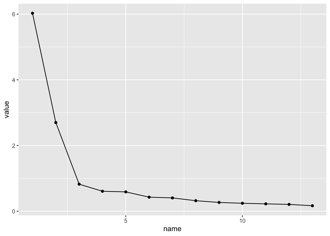

A more nuanced approach to this problem is parallel analysis. This generates random data from your dataset to replicate this process more realistically to your own data. By default, this uses Pearson correlations, but you have the option to use cor = "poly" in order to use polychoric correlations. While polychoric correlations are “more technically correct” for likert style items, the results are often the same and polychoric correlation can be a hassle (sometimes they take too long, or don’t work at all).

psych::fa.parallel(sps)

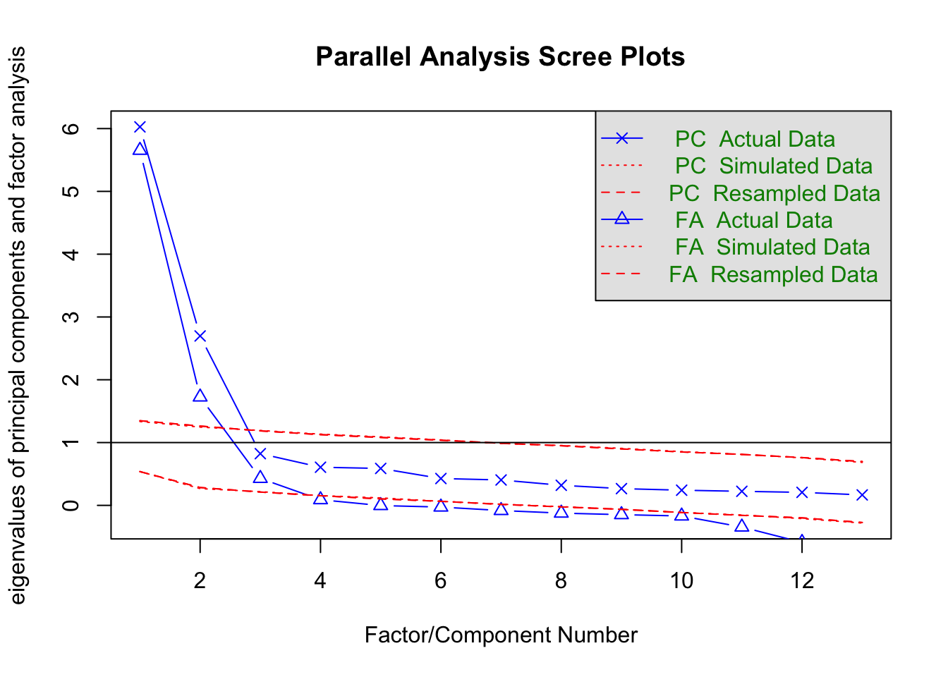
## Parallel analysis suggests that the number of factors =  3  and the number of components =  2

#psych::fa.parallel(sps,cor = "poly") #Does the same but based on polychoric rather than pearson correlations.

The analysis suggests the extraction of 2 components or 3 factors. We won’t go into the distinction between components and factors, as it is not consequential for our purposes.

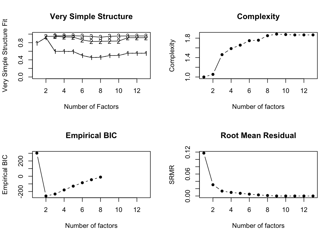
Finally, there is an array of other techniques, like Very Simple Structure complexity (VSS), the Minimum Average Partial method (MAP) and Bayesian Information Criterion (BIC). Those can be analyzed using the nfactors() command.

psych::nfactors(sps)

## 
## Number of factors
## Call: vss(x = x, n = n, rotate = rotate, diagonal = diagonal, fm = fm, 
##     n.obs = n.obs, plot = FALSE, title = title, use = use, cor = cor)
## VSS complexity 1 achieves a maximimum of 0.92  with  2  factors
## VSS complexity 2 achieves a maximimum of 0.95  with  3  factors
## The Velicer MAP achieves a minimum of 0.03  with  3  factors 
## Empirical BIC achieves a minimum of  -258.49  with  2  factors
## Sample Size adjusted BIC achieves a minimum of  -32.34  with  4  factors
## 
## Statistics by number of factors 
##    vss1 vss2   map dof   chisq     prob sqresid  fit RMSEA  BIC SABIC complex
## 1  0.79 0.00 0.053  65 8.4e+02 1.0e-135    9.53 0.79 0.195  469 674.9     1.0
## 2  0.92 0.95 0.035  53 2.9e+02  9.7e-34    2.42 0.95 0.118  -19 149.4     1.1
## 3  0.60 0.95 0.033  42 7.6e+01  9.1e-04    1.81 0.96 0.051 -165 -32.0     1.5
## 4  0.60 0.93 0.051  32 5.0e+01  2.1e-02    1.60 0.97 0.042 -134 -32.3     1.6
## 5  0.59 0.93 0.069  23 3.3e+01  8.5e-02    1.44 0.97 0.037 -100 -26.7     1.7
## 6  0.50 0.86 0.099  15 1.6e+01  3.7e-01    1.27 0.97 0.016  -70 -22.5     1.7
## 7  0.45 0.83 0.122   8 7.2e+00  5.1e-01    0.99 0.98 0.000  -39 -13.5     1.8
## 8  0.46 0.83 0.155   2 1.4e+00  5.1e-01    0.99 0.98 0.000  -10  -3.8     1.9
## 9  0.50 0.84 0.221  -3 2.0e-04       NA    1.05 0.98    NA   NA    NA     1.9
## 10 0.50 0.84 0.311  -7 2.4e-06       NA    1.06 0.98    NA   NA    NA     1.9
## 11 0.55 0.92 0.483 -10 5.8e-09       NA    1.05 0.98    NA   NA    NA     1.9
## 12 0.55 0.92 1.000 -12 2.7e-09       NA    1.04 0.98    NA   NA    NA     1.9
## 13 0.55 0.92    NA -13 2.7e-09       NA    1.04 0.98    NA   NA    NA     1.9
##     eChisq    SRMR  eCRMS eBIC
## 1  6.8e+02 1.2e-01 0.1284  303
## 2  4.7e+01 3.1e-02 0.0373 -258
## 3  8.9e+00 1.3e-02 0.0183 -233
## 4  4.7e+00 9.7e-03 0.0152 -180
## 5  2.7e+00 7.4e-03 0.0135 -130
## 6  1.2e+00 5.0e-03 0.0114  -85
## 7  4.2e-01 2.9e-03 0.0091  -46
## 8  7.8e-02 1.3e-03 0.0079  -11
## 9  1.1e-05 1.5e-05     NA   NA
## 10 1.8e-07 1.9e-06     NA   NA
## 11 2.7e-10 7.5e-08     NA   NA
## 12 1.4e-10 5.3e-08     NA   NA
## 13 1.4e-10 5.3e-08     NA   NA

A correlation matrix can also help you decide how many factors you want to extract. Here, bigger circles represent bigger correlations (red = negative, blue = positive).

# install.packages("corrplot")

sps %>% #data
  cor() %>% #generate correlations
  corrplot::corrplot(tl.col = "black",order = "hclust") #visualize. Hclust orders correlations.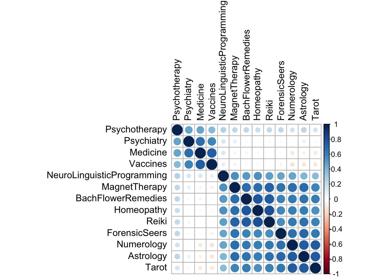

In this case, we see that there are two groups of items that are unrelated with each other, but correlated within each group. It seems like science and pseudoscience represent independent factors rather than two ends in a single continuum.

Fig 2. Two independent factors

Based on our theoretical intuitions and all of the evidence we have seen, it makes sense to try and extract two factors. How would we go about doing that?

5.5.3 How do we extract factors?

We are finally ready to run factor analysis. So far we figured out that our data is factorizable and that 2 factors are likely the optimum.

Factor extraction means generating linear combinations of the variables (13 items) to generate factors (2 in our case). A linear combination is just a weighted average of the scores of each participant for each item, to represent the factors. The weights are called factor loadings and represent the correlation between the item and the factor.

We still need to make one more decision before extracting our factors. Which factor extraction method will we use? Here are some and their use cases.

Method	Use case
Principal Components Analysis (PCA)	Is not “really” factor analysis, but as SPSS default, it is also a default in a lot of published research.
Principal Axis Factoring (PAF)	Usually used with normal and continuous data.
Maximum Likelihood (ML)	Usually used with normal and continuous data.
Unweighted Least Squares (ULS/MinRes)	A more robust variant that works better with non-normal likert type data
Ordinary Least Squares (OLS)	A more robust variant that works better with non-normal likert type data
Weighted Least Squares (WLS)	A more robust variant that works better with non-normal likert type data

All of these are available in the fa() function, using the fm = argument. PCA is not available in fa() and can be accessed using principal(). Our default recommendation for likert items is the ULS factorization method (fm = "uls"). This is fa’s default.

principal(r = sps,nfactors = 2)

## Principal Components Analysis
## Call: principal(r = sps, nfactors = 2)
## Standardized loadings (pattern matrix) based upon correlation matrix
##                              RC1   RC2   h2   u2 com
## Psychiatry                  0.04  0.83 0.69 0.31 1.0
## Astrology                   0.85 -0.01 0.73 0.27 1.0
## Medicine                   -0.08  0.90 0.81 0.19 1.0
## Psychotherapy               0.26  0.66 0.51 0.49 1.3
## ForensicSeers               0.79  0.02 0.62 0.38 1.0
## MagnetTherapy               0.84  0.04 0.71 0.29 1.0
## NeuroLinguisticProgramming  0.63  0.22 0.44 0.56 1.2
## Tarot                       0.80 -0.06 0.64 0.36 1.0
## Numerology                  0.84 -0.06 0.71 0.29 1.0
## BachFlowerRemedies          0.84  0.03 0.71 0.29 1.0
## Homeopathy                  0.83  0.03 0.69 0.31 1.0
## Reiki                       0.85  0.05 0.72 0.28 1.0
## Vaccines                   -0.10  0.85 0.73 0.27 1.0
## 
##                        RC1  RC2
## SS loadings           6.01 2.71
## Proportion Var        0.46 0.21
## Cumulative Var        0.46 0.67
## Proportion Explained  0.69 0.31
## Cumulative Proportion 0.69 1.00
## 
## Mean item complexity =  1
## Test of the hypothesis that 2 components are sufficient.
## 
## The root mean square of the residuals (RMSR) is  0.04 
##  with the empirical chi square  89.82  with prob <  0.0012 
## 
## Fit based upon off diagonal values = 0.99

fit = fa(r = sps,nfactors = 2,fm = "uls")

## Loading required namespace: GPArotation

fit

## Factor Analysis using method =  uls
## Call: fa(r = sps, nfactors = 2, fm = "uls")
## Standardized loadings (pattern matrix) based upon correlation matrix
##                             ULS1  ULS2   h2   u2 com
## Psychiatry                  0.07  0.74 0.56 0.44 1.0
## Astrology                   0.84 -0.03 0.70 0.30 1.0
## Medicine                   -0.05  0.91 0.83 0.17 1.0
## Psychotherapy               0.27  0.54 0.36 0.64 1.5
## ForensicSeers               0.76  0.00 0.57 0.43 1.0
## MagnetTherapy               0.82  0.02 0.68 0.32 1.0
## NeuroLinguisticProgramming  0.59  0.18 0.37 0.63 1.2
## Tarot                       0.77 -0.07 0.60 0.40 1.0
## Numerology                  0.82 -0.08 0.68 0.32 1.0
## BachFlowerRemedies          0.82  0.01 0.68 0.32 1.0
## Homeopathy                  0.81  0.01 0.65 0.35 1.0
## Reiki                       0.83  0.03 0.69 0.31 1.0
## Vaccines                   -0.07  0.79 0.63 0.37 1.0
## 
##                       ULS1 ULS2
## SS loadings           5.66 2.34
## Proportion Var        0.44 0.18
## Cumulative Var        0.44 0.62
## Proportion Explained  0.71 0.29
## Cumulative Proportion 0.71 1.00
## 
##  With factor correlations of 
##       ULS1  ULS2
## ULS1  1.00 -0.01
## ULS2 -0.01  1.00
## 
## Mean item complexity =  1.1
## Test of the hypothesis that 2 factors are sufficient.
## 
## df null model =  78  with the objective function =  8.94 with Chi Square =  2770.09
## df of  the model are 53  and the objective function was  0.93 
## 
## The root mean square of the residuals (RMSR) is  0.04 
## The df corrected root mean square of the residuals is  0.05 
## 
## The harmonic n.obs is  316 with the empirical chi square  46.56  with prob <  0.72 
## The total n.obs was  316  with Likelihood Chi Square =  286.33  with prob <  9.7e-34 
## 
## Tucker Lewis Index of factoring reliability =  0.872
## RMSEA index =  0.118  and the 90 % confidence intervals are  0.105 0.132
## BIC =  -18.73
## Fit based upon off diagonal values = 0.99
## Measures of factor score adequacy             
##                                                   ULS1 ULS2
## Correlation of (regression) scores with factors   0.97 0.94
## Multiple R square of scores with factors          0.94 0.89
## Minimum correlation of possible factor scores     0.88 0.78

Here we run factor analysis and save the results in an object called fit.

Before interpreting the results, we should take a look at rotation, the last step, which will improve the interpretability of the results and separate the two factors more clearly.

5.5.4 Rotation?

As with factor extraction, there is a large array of rotation methods. The only thing that really matters is whether you are choosing an oblique or an orthogonal rotation. Orthogonal means that you are forcing the factors to be perfectly uncorrelated ($r = 0$), whereas in oblique rotation the factors are allowed to correlate and the correlation between the factors is calculated.

This should be decided on the basis of theory and empirically–whether your items are actually correlated across factors. Do note, though, that in psychology, factors are almost always correlated. I usually start with an oblique rotation and keep it if the factors are correlated, and I might try an orthogonal rotation if they are unrelated. The rotation is chosen with the rotate = parameter within fa().

Some orthogonal rotations: “varimax”, “quartimax”, “bentlerT”, “equamax”, “varimin”, “geominT” and “bifactor” Some oblique rotations: “Promax”, “promax”, “oblimin” (default), “simplimax”, “bentlerQ,”geominQ” and “biquartimin” and “cluster”.

Let us see our rotated factor loading matrix and see how the items are arranged.

fit = fa(r = sps,nfactors = 2,fm = "uls",rotate = "oblimin")
print.psych(fit,cut=.3,sort=T)

## Factor Analysis using method =  uls
## Call: fa(r = sps, nfactors = 2, rotate = "oblimin", fm = "uls")
## Standardized loadings (pattern matrix) based upon correlation matrix
##                            item  ULS1  ULS2   h2   u2 com
## Astrology                     2  0.84       0.70 0.30 1.0
## Reiki                        12  0.83       0.69 0.31 1.0
## MagnetTherapy                 6  0.82       0.68 0.32 1.0
## BachFlowerRemedies           10  0.82       0.68 0.32 1.0
## Numerology                    9  0.82       0.68 0.32 1.0
## Homeopathy                   11  0.81       0.65 0.35 1.0
## Tarot                         8  0.77       0.60 0.40 1.0
## ForensicSeers                 5  0.76       0.57 0.43 1.0
## NeuroLinguisticProgramming    7  0.59       0.37 0.63 1.2
## Medicine                      3        0.91 0.83 0.17 1.0
## Vaccines                     13        0.79 0.63 0.37 1.0
## Psychiatry                    1        0.74 0.56 0.44 1.0
## Psychotherapy                 4        0.54 0.36 0.64 1.5
## 
##                       ULS1 ULS2
## SS loadings           5.66 2.34
## Proportion Var        0.44 0.18
## Cumulative Var        0.44 0.62
## Proportion Explained  0.71 0.29
## Cumulative Proportion 0.71 1.00
## 
##  With factor correlations of 
##       ULS1  ULS2
## ULS1  1.00 -0.01
## ULS2 -0.01  1.00
## 
## Mean item complexity =  1.1
## Test of the hypothesis that 2 factors are sufficient.
## 
## df null model =  78  with the objective function =  8.94 with Chi Square =  2770.09
## df of  the model are 53  and the objective function was  0.93 
## 
## The root mean square of the residuals (RMSR) is  0.04 
## The df corrected root mean square of the residuals is  0.05 
## 
## The harmonic n.obs is  316 with the empirical chi square  46.56  with prob <  0.72 
## The total n.obs was  316  with Likelihood Chi Square =  286.33  with prob <  9.7e-34 
## 
## Tucker Lewis Index of factoring reliability =  0.872
## RMSEA index =  0.118  and the 90 % confidence intervals are  0.105 0.132
## BIC =  -18.73
## Fit based upon off diagonal values = 0.99
## Measures of factor score adequacy             
##                                                   ULS1 ULS2
## Correlation of (regression) scores with factors   0.97 0.94
## Multiple R square of scores with factors          0.94 0.89
## Minimum correlation of possible factor scores     0.88 0.78

The first part of the output gives us what we want the most: our precious factor loading matrix. We use the print.psych command that allows us to hide small factor loadings (< .3) and sort the factor loading matrix. This simplifies readability and interpretability. We see a nice pattern where all items load highly on their respective factor and have low or null loadings on the different factor. (Try removing the cut = .3 to see all factor loadings).

We don’t have many problems in this data but here are a few potential problems:

Items with very low loadings in all factors: The item doesn't accurately represent any of the factors

Item that loads highly in a factor where it "shouldn't" belong: The item for some reason correlates more with theoretically unrelated (rather than related) items.

Items with high loadings in two factors: The item lacks discriminant validity. It measures two things instead of one.

The sign of the loading is off: A positive sign in the factor loading implies that the item is directly related with the factor. Negative loadings imply that there is an inverse relation. For example: "I feel sad" might load negatively in a measure of happiness.

The second part of the output gives us how much of the original variance of the 13 items is preserved on our two factor solution. We see that the first factor explains 44% and the second one 18% for a combined 62% of the variance. Take a second to evaluate how good a deal this is. You transformed 13 items into 2 variables (15%), but kept 62% of the information.

After that we have our factor intercorrelations. In this case the factors are correlated at -.01, meaning the factors are practically orthogonal. We could re-run our analysis using orthogonal rotation (e.g. Varimax). What this means is that trusting science doesn’t mean you will distrust pseudoscience. Believing pseudoscience doesn’t mean you distrust science.

We can visualize our results using the plot command. Each axis represents a factor, and points represent items with x and y loadings in each axis. Items on the axis load on a single factor. Items near the origin have loadings that are too low. Items far from the axis, standing in no-man’s land have worse discriminant validity.

plot(fit)

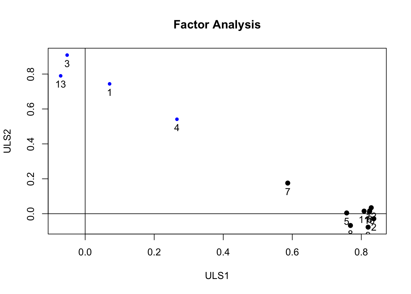
Here, we see that items 4 (psychotherapy) and 7 (neurolinguistic programming) are not as close to their respective axes, indicating small cross loadings. Most other items are right on the axes, meaning they load more univocally on their respective factors.

Finally, let’s use factor scores to see how the 316 people land on these quadrants. BTW, factor scores are the factor analysis cousin of simple composites. They take into account factor loadings to calculate some sort of weighted average of the level of each factor for each person. There are several ways to calculate them, and we won’t go into detail here, but read this if you are interested.

Since factor scores have means 0, we can use that as a mean split to categorize our participants.

fit$scores %>% as.data.frame() %>% 
  rename(Pseudoscience = ULS1,
         Science = ULS2) %>% 
  mutate(Category = case_when(Science>0 & Pseudoscience>0 ~ "Believes all",
                              Science<0 & Pseudoscience<0 ~ "Skeptic",
                              Science>0 & Pseudoscience<0 ~ "Only Science",
                              Science<0 & Pseudoscience>0 ~ "Only Pseudoscience")) %>% 
  ggplot(aes(Science,Pseudoscience,col=Category))+
  geom_point()+
  geom_hline(yintercept = 0)+
  geom_vline(xintercept = 0)+
  labs(title = "Belief in science is unrelated to belief in pseudoscience")+
  theme(legend.position = "bottom")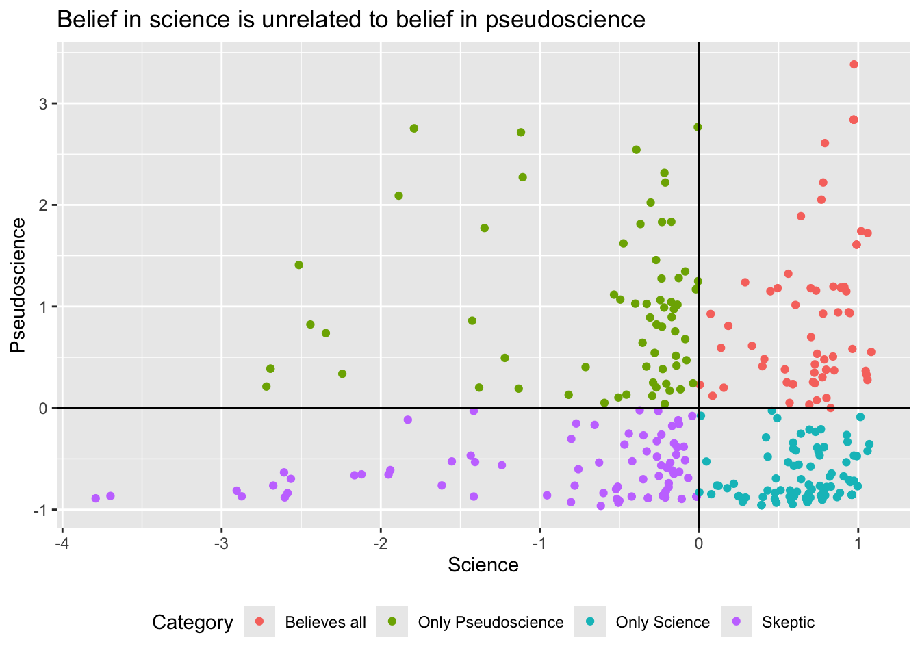

What did we learn? That factor analysis is a lot of fun. You have enough information to impress your crush next time you see him or her at a party. Kidding aside, Factor Analysis is a powerful technique that allows you to analyze the interrelations between items. It analyzes the pattern of responses people give to your items to find a way to compress the information in a large number of items into a smaller number of factors while retaining the maximum amount of information. This helps us understand how our measure works and justifies the way we use concrete items to refer to unobservable constructs.

Here is your checklist:

Are the items correlated enough? Take a glance at the correlations, see if Bartlett’s Sphericity Test (cortest.bartlett) is significant, and Kaiser Meyer Olkin’s Sampling Adequacy Measure is… well, adequate (KMO).
Decide how many factors you want to extract. Use a combination of theory, visual inspection of the scree plot (data %>% cor %>% eigen), and more advanced methods like parallel analysis (fa.parallel) to decide.
Choose a factor extraction method (most likely unweighted least squares fa(data,nfactors,fm='uls) if you are using likert style items).
Choose whether you want orthogonal (e.g. rotate = "varimax"), or oblique (e.g. rotate = "oblimin") rotation. Usually factors are related enough to justify oblique rotation, but if upon inspection factors are not correlated, orthogonal rotation might be simpler.
Inspect your factor loading matrix to see how good are your items at representing the latent factors.
See how much information you could retain.
Celebrate because you are finally done!

5.6 Review: End Notes

Today, we covered:

What an outlier is, where outliers come from, and the three problems they cause
Finding and handling univariate outliers: out-of-bounds values, boxplots, and the z-score method
Multivariate outliers with Mahalanobis distance
What Cronbach’s alpha actually measures, how to compute it, and what it is not
Factor analysis: whether items are factorable, how many factors to extract, extraction methods, and rotation

5.6.1 Quick reference: outliers and psychometrics

Finding and handling outliers

Function	What It Does
`geom_boxplot()`	A quick visual check–points beyond the whiskers are candidate outliers
`filter()`	Finds out-of-bounds values, e.g. `filter(efficacy < 1)`
`ifelse()`	Recodes bad values as missing: `ifelse(efficacy < 1, NA, efficacy)`
`scale()`	Converts a variable to z-scores. The conventional cutoff is beyond +/- 3
`mahalanobis()`	A multivariate distance–like a z-score, but across several variables at once, and taking their correlations into account
`MO_Detection()`	The custom function we wrote, which computes Mahalanobis distances, applies a chi-squared cutoff, and returns the data without the outliers

Reliability

Function	What It Does
`alpha()`	From `psych`. Computes Cronbach’s alpha and a great deal else
`alpha_table()`	The function we wrote, which pulls the useful parts of `alpha()` into a readable table
`$total$raw_alpha`	Where the headline alpha value lives inside the `alpha()` output

Standards: .70 acceptable, .80 good, .90 great. Alpha rises both when items correlate more strongly and when you simply add more items–so a high alpha does not by itself mean your items are strongly related.

Factor analysis

Function	What It Does
`KMO()`	Sampling adequacy–is there enough shared variance to factor at all? Above .80 is good
`cortest.bartlett()`	Tests the correlation matrix against an identity matrix. You want this significant
`cor() %>% eigen()`	Eigenvalues. The old rule of thumb is to keep factors with eigenvalues above 1
`fa.parallel()`	Parallel analysis–a more defensible way to decide how many factors to extract
`nfactors()`	Runs several other selection criteria at once (VSS, MAP, BIC)
`fa()`	Runs the factor analysis. `fm = "uls"` is a good default for Likert items
`principal()`	Principal Components Analysis, which is not quite factor analysis
`print.psych(cut=.3)`	Prints the loading matrix, hiding small loadings so the pattern is readable

Rotation: orthogonal (e.g. "varimax") forces factors to be uncorrelated; oblique (e.g. "oblimin", the default) lets them correlate. In psychology, factors usually do.

5.6.2 Feedback

As a learner, your superpower is knowing what is and isn’t working for your learning. If you have 2 minutes, we would love if you shared your superpower with us!

Scan the QR code below with your phone to provide brief feedback on this workshop:

5.6.3 Some useful resources to continue your learning

A useful resource, in my opinion, is the stackoverflow website. Because this is a general-purpose resource for programming help, it will be useful to use the R tag ([R]) in your queries. A related resource is the statistics stackexchange, which is like Stack Overflow but focused more on the underlying statistical issues.

One of the best resources for learning how to use R well, in a “tidy” way, is R for Data Science (R4DS).

5.6.4 What’s an R Markdown again?

This is the main kind of document that I use in RStudio, and I think its one of the primary advantage of RStudio over base R console. R Markdown allows you to create a file with a mix of R code and regular text, which is useful if you want to have explanations of your code alongside the code itself. This document, for example, is an R Markdown document. It is also useful because you can export your R Markdown file to an html page or a pdf, which comes in handy when you want to share your code or a report of your analyses to someone who doesn’t have R. If you’re interested in learning more about the functionality of R Markdown, you can visit this webpage

R Markdowns use chunks to run code. A chunk is designated by starting with {r}and ending with This is where you will write your code. A new chunk can be created by pressing COMMAND + ALT + I on Mac, or CONTROL + ALT + I on PC.

You can run lines of code by highlighting them, and pressing COMMAND + ENTER on Mac, or CONTROL + ENTER on PC. If you want to run a whole chunk of code, you can press COMMAND + ALT + C on Mac, or ALT + CONTROL + ALT + C on PC. Alternatively, you can run a chunk of code by clicking the green right-facing arrow at the top-right corner of each chunk. The downward-facing arrow directly left of the green arrow will run all code up to that point.